UDF for calculating hillshade seems not to process all the chunks

Hi all,

I am working on a UDF that reproduces the gdal function to create the hillshade.

First, I get the DEM

eoconn = openeo.connect('https://openeo.dataspace.copernicus.eu/', auto_validate=False)
eoconn.authenticate_oidc()

dem_datacube = eoconn.load_collection(
    "COPERNICUS_30",
    spatial_extent={'west':11.241593,
                    'east':11.444267,
                    'south':46.914255,
                    'north':46.992429,
                    'crs':4326},
    bands=["DEM"]
)

Then, I apply the udf

udf_path="./udf-hillshade.py"
hillshade_func = openeo.UDF.from_file(udf_path, context={"from_parameter": "context"})

hillshade = dem_datacube.apply(process=hillshade_func) 

where the udf is defined in this way

import openeo 
from openeo.udf.debug import inspect
from openeo.udf import XarrayDataCube

import math
import numpy as np 
import xarray as xr 
from skimage.restoration import inpaint


def apply_datacube(cube: XarrayDataCube, 
                   context: dict) -> XarrayDataCube:
    
    """
    UDF to get the hillshade, i.e., a shaded relief map.
    It takes the illumination angles as input, i.e.,
        altitude of the sun (default 315 degrees: the terrain is lit as if the 
                             light source is coming from the upper left) 
        azimuth of the sun (default 45 degrees: the light is pitched 45 degrees
                            between the horizon and directly overhead) 
        
    First, the slope and aspect are calculated by following Horn (1981).
    
    Input and output datacube have the same dimensions.
    """
    
    altitude = 45
    azimuth = 315
    nodataval = 255
    
    # conversion from degrees to radians
    deg2rad = 180/np.pi
    
    # zenith angle of the sun calculated from the altitude
    zenith_rad = (90 - altitude)/deg2rad
    # zenith angle of the sun calculated from the altitude
    azimuth_rad = azimuth/deg2rad
    
    # load the datacube
    array = cube.get_array()
    data_array = array.values[0]
        
    # get the coodinates of the datacube
    xmin = array.coords['x'].min()
    xmax = array.coords['x'].max()
    ymin = array.coords['y'].min()
    ymax = array.coords['y'].max()
    
    coord_x = np.linspace(start = xmin, 
                          stop = xmax,
                          num = array.shape[-2])
    
    coord_y = np.linspace(start = ymin, 
                          stop = ymax,
                          num = array.shape[-1])
    
    # get the datacube spatial resolution
    resolution = array.coords['x'][-1] - array.coords['x'][-2]
    
    # Calculate gradients
    dz_dx = ((data_array[:-2, 2:] + 2 * data_array[1:-1, 2:] + data_array[2:, 2:]) -
            (data_array[:-2, :-2] + 2 * data_array[1:-1, :-2] + data_array[2:, :-2]))/(8 * resolution.values)
    dz_dy = ((data_array[2:, :-2] + 2 * data_array[2:, 1:-1] + data_array[2:, 2:]) -
            (data_array[:-2, :-2] + 2 * data_array[:-2, 1:-1] + data_array[:-2, 2:])) / (8 * resolution.values)
    
  
    # Compute slope and aspect
    slope = np.arctan(np.sqrt(dz_dx**2 + dz_dy**2)) 
    aspect = np.arctan2(dz_dy, -dz_dx)
    aspect = np.where(aspect < np.pi/2, np.pi/2 - aspect, 5*np.pi/2 - aspect)

    # Compute hillshade
    hillshade = (np.cos(zenith_rad) * np.cos(slope) +
                  np.sin(zenith_rad) * np.sin(slope) * np.cos(azimuth_rad - aspect))
    hillshade = np.clip(hillshade, 0, 1)
    

    # Scale to 0-255
    hillshade = nodataval * hillshade
    hillshade[hillshade<0] = 0
    hillshade[slope==0] = 0
    
    # round to integers
    hillshade = np.round(hillshade)
    
    # Create output array and insert hillshade values
    output = np.zeros_like(data_array) + nodataval
    output[1:-1, 1:-1] = hillshade


    # Create a mask for the 255 values
    mask = (output == 255).astype(np.uint8)
    
    # Replace the 255 values using biharmonic inpainting
    interpolated_array = inpaint.inpaint_biharmonic(output, mask)
    interpolated_array = interpolated_array.astype(np.uint8)
    
    # predicted datacube: same dimensions as the input datacube
    predicted_cube = xr.DataArray(interpolated_array, 
                                  dims=['x', 'y'],                             
                                  coords=dict(x=coord_x, y=coord_y))
    
    return XarrayDataCube(predicted_cube)

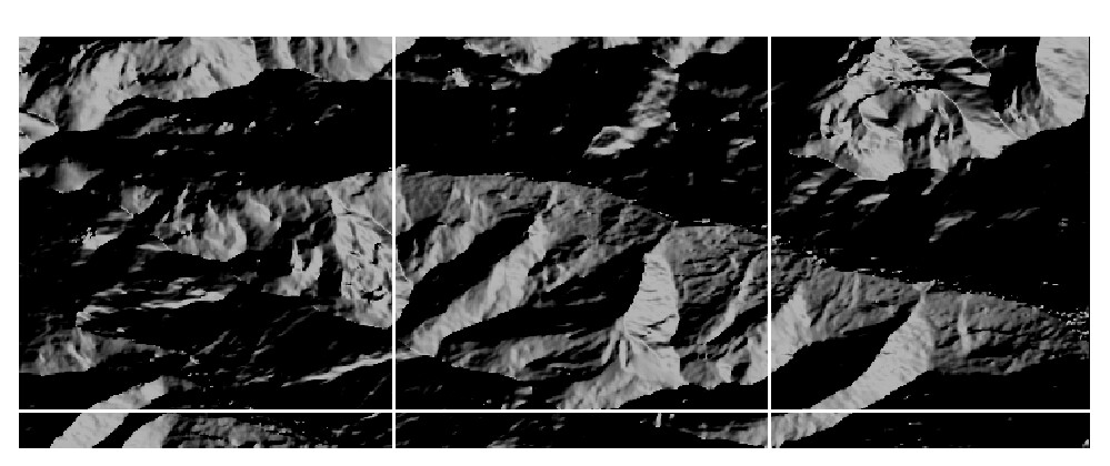
I have tested the UDF and it is working. However, I needed to add something to interpolate missing values on the edges. When I add this last step about the inpainting - last lines of the code-, it returns a partial output

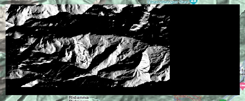
You can see that sume chunks seem not to be processed. Can you help and tell me why?

Thanks,
Valentina

I’m investigating.

One thing I noticed is that inpaint.inpaint_biharmonic returns a floating point ndarray of [0-1] values regardless of the input it received ([0-255] uint8 in your case).
My initial guess is that this behavior is causing some issues when we try to stitch tiles together.

So I would try to convert the inpaint output back to 0-255 uint8 first

Hi Stefaan,

thanks for your answer.
Not sure I got your suggestion.
The input to inpaint_biharmonic, i.e., the array called “output” should be float32 if I am not wrong, while the mask is [0-1] . Anyway, if I keep the mask as bool

    mask = (output == 255)

nothing changes.

ALso, I have tried to remove this line of code

    interpolated_array = interpolated_array.astype(np.uint8)

but the problem still remains.

yes, I’m still quite confused by the behavior of inpaint.inpaint_biharmonic at the moment. And I also have no idea yet how using it makes output to disappear.

In any case: if I understand correctly, you are using that inpaint functionality to fill in the one pixel no-data border of your tile.
I would consider doing that in a more low-tech approach, e.g. output[0, :] = output[1, :] etc
You know in advance which pixels you want to fill in anyway and it will be a more efficient too I guess.

next hypothesis: inpaint.inpaint_biharmonic get as input output of dtype “float32”
possibly containing nodata values and inpaint.inpaint_biharmonic can not handle that

Yes, indeed a simple replacement could be a workaround.
Still, I think that it is a little bit weird that this behavior is happening only for some chunks. Indeed, if I use the same function without the inpainting, the result looks good and there aren’t no data

The inpainting was intended to remove the no data stripes at the borders, maybe a solution could be using apply_neighborhood instead of apply as suggested now by @michele.claus

Still, very strange that the inpainting is correct for some of the chunks only (see image above)…

I did some more testing and the lack of no-data handling in interpolated_array = inpaint.inpaint_biharmonic(output, mask) is the problem here. If one non-masked pixel of output (dtype float32 in your use case) is numpy.nan, then the whole of interpolated_array becomes no-data.

If I change the mask in your code as follows, inpaint.inpaint_biharmonic will not fail that way:

    mask = (output == 255) | np.isnan(output)

(Note that all that astype() casting you are currently doing is not necessary I think)

Some more explanation of what is happening here:

dem_datacube.apply(process=hillshade_func)

while apply is officially a point-process, the data is still processed in tiles or chunks in the UDF: the cube input your apply_datacube is basically a (sub)cube, not a single pixel. The backend automatically chunks the whole data cube in 512x512 chunks for you and passes these (parallelized) to apply_datacube.
However, as your spatial extent does not exactly matches a 512x512 grid, some chunks are padded with no-data.
In your original use case, you have 6 chunks in total, but four of them (at right/bottom) are padded as such.
inpaint.inpaint_biharmonic does not handle that properly and returns a full-nodata tile for those four chunks.

1 Like

FYI: discussion on NaN support in scikit-image: Add support for image data with NaNs · Issue #1624 · scikit-image/scikit-image · GitHub

Thank you very much :slight_smile:

Still, based on your experience is it better this way by using apply or would you suggest apply neighbor?
I did not manage btw to use it, since there is a problem with the dimensions when using the same udf… I will give another try soon

I haven’t looked into the hillshade implementation details, but I can imagine that there are border artifacts (not only because of the gap filling, but also because of incomplete shade calculations).
If these border artifacts are indeed a problem you should indeed switch to apply_neighborhood where the chunking will be done with overlap (e.g. 8 or 16 pixels overlap at the borders). That should cover the short-range shade calculations. And you wont need a gap filling step at the borders, because that will be automatically covered through the overlap handling.

if the border artifacts are not a concerning problem, you can of course stick to apply

Hi Stefaan,

thanks a lot for your suggestion. Just to let you know and share it with other interested users, I have managed to run the same with apply_neighborhood and I got a correct result.

I share the code here (maybe something could be improved but it works…)


def apply_datacube(cube: XarrayDataCube, 
                   context: dict) -> XarrayDataCube:
    
    """
    UDF to get the hillshade, i.e., a shaded relief map.
    It takes the illumination angles as input, i.e.,
        altitude of the sun (default 315 degrees: the terrain is lit as if the 
                             light source is coming from the upper left) 
        azimuth of the sun (default 45 degrees: the light is pitched 45 degrees
                            between the horizon and directly overhead) 
        
    First, the slope and aspect are calculated by following Horn (1981).
    
    Input and output datacube have the same dimensions.
    """
    
    altitude = 45
    azimuth = 315
    nodataval = 255
    
    # conversion from degrees to radians
    deg2rad = 180/np.pi
    
    # zenith angle of the sun calculated from the altitude
    zenith_rad = (90 - altitude)/deg2rad
    # zenith angle of the sun calculated from the altitude
    azimuth_rad = azimuth/deg2rad
    
    # load the datacube
    array = cube.get_array()
    # inspect(array.dims)
    array = array.transpose("t", "bands", "y", "x")
    input_shape = array.shape

    data_array = array.values[0,0,:,:]
        
    # get the coodinates of the datacube
    xmin = array.coords['x'].min()
    xmax = array.coords['x'].max()
    ymin = array.coords['y'].min()
    ymax = array.coords['y'].max()
    
    coord_x = np.linspace(start = xmin, 
                          stop = xmax,
                          num = array.shape[-2])
    
    coord_y = np.linspace(start = ymin, 
                          stop = ymax,
                          num = array.shape[-1])
    
    # get the datacube spatial resolution
    resolution = array.coords['x'][-1] - array.coords['x'][-2]
    
    # Calculate gradients
    dz_dx = ((data_array[:-2, 2:] + 2 * data_array[1:-1, 2:] + data_array[2:, 2:]) -
            (data_array[:-2, :-2] + 2 * data_array[1:-1, :-2] + data_array[2:, :-2]))/(8 * resolution.values)
    dz_dy = ((data_array[2:, :-2] + 2 * data_array[2:, 1:-1] + data_array[2:, 2:]) -
            (data_array[:-2, :-2] + 2 * data_array[:-2, 1:-1] + data_array[:-2, 2:])) / (8 * resolution.values)
    
  
    # Compute slope and aspect
    slope = np.arctan(np.sqrt(dz_dx**2 + dz_dy**2)) 
    aspect = np.arctan2(dz_dy, -dz_dx)
    aspect = np.where(aspect < np.pi/2, np.pi/2 - aspect, 5*np.pi/2 - aspect)

    # Compute hillshade
    hillshade = (np.cos(zenith_rad) * np.cos(slope) +
                  np.sin(zenith_rad) * np.sin(slope) * np.cos(azimuth_rad - aspect))
    hillshade = np.clip(hillshade, 0, 1)
    

    # Scale to 0-255
    hillshade = nodataval * hillshade
    hillshade[hillshade<0] = 0
    hillshade[slope==0] = 0
    
    # round to integers
    hillshade = np.round(hillshade)
    
    # Create output array and insert hillshade values
    output = np.zeros_like(data_array) + nodataval
    output[1:-1, 1:-1] = hillshade


    coord_t = cube.get_array().coords['t'].values
    band = cube.get_array().coords['bands'].values

    
    # predicted datacube: same dimensions as the input datacube
    predicted_cube = xr.DataArray(output.reshape(input_shape),  # Reshape the output to the original shape (bands, y, x)
                                  dims=['t','bands','y', 'x'],                             
                                  coords=dict(t=coord_t, bands=band, x=coord_x, y=coord_y))


    return XarrayDataCube(predicted_cube)
 

called in the main script in this way

# Load the UDF from a file.
udf_path="./udf-hillshade.py"

hillshade_func = openeo.UDF.from_file(udf_path, context={"from_parameter": "context"})


# Apply the UDF to the data cube.
hillshade = dem_datacube.apply_neighborhood(
    hillshade_func,
    size=[
        {"dimension": "x", "value": 224, "unit": "px"},
        {"dimension": "y", "value": 224, "unit": "px"},
    ],
    overlap=[
        {"dimension": "x", "value": 16, "unit": "px"},
        {"dimension": "y", "value": 16, "unit": "px"}
    ],
)
2 Likes